Sunday, August 11, 2013

Spring JDBCTemplate Vs Hibernate Performance + JPA & Caching

Spring JDBCTemplate Vs Hibernate Performance

If you do all you can to make Spring JDBCTemplate / Hibernate implementations very fast, the JDBC template will probably be a bit faster, because it doesn't have the overhead that Hibernate has, but it will probably take much more time and lines of code to implement.

Hibernate has its learning curve, and you have to understand what happens behind the scenes, when to use projections instead of returning entities, etc. But if you master it, you'll gain much time and have cleaner and simpler code than with a JDBC-based solution.

In 95% of the cases, Hibernate is fast enough, or even faster than non-optimized JDBC code. For the 5% left, nothing forbids you to use something else, like Spring-JDBC for example. Both solutions are not mutually exclusive.

Hibernate

Hibernate is not intended for batch-jobs, it is an anti patterns of O/R Mapper usage.  Even the Hibernate documentation warns to not do that. Batch processing often can be much more easily done by a single clever SQL statement instead via O/R mappers which need a bunch of statements to do the same. Not because they are bad, but because they have not been built for this use case. Data is always by default loaded lazyly in Hibernate.

One of the common problems of people that start using Hibernate is performance, if you don’t have much experience in Hibernate you will find how quickly your application becomes slow. If you enable sql traces, you would see how many queries are sent to database that can be avoided with little Hibernate knowledge. Good use of Hibernate Cache to avoid amount of traffic between your application and database.

JPA + Spring

If you are using spring and JPA, it is very likely that you utilize ehcache (or another cache provider). And you do that in two separate scenarios: JPA 2nd level cache and spring method caching.

When you configure your application, you normally set the 2nd level cache provider of your JPA provider (hibernate, in my case) and you also configure spring with the “cache” namespace. Everything looks OK and you continue with the project. But there’s a caveat. If you follow the most straightforward way, you get two separate cache managers which load the same cache configuration file. This is not bad per-se, but it is something to think about – do you really need two cache manager and the problems that may arise from this

JPA & Caching

Caching is the most important performance optimization technique. There are many things that can be cached in persistence, objects, data, database connections, database statements, query results, meta-data, relationships, to name a few. Caching in object persistence normally refers to the caching of objects or their data.

Caching also influences object identity, that is that if you read an object, then read the same object again you should get the identical object back (same reference).

JPA 1.0 does not define a shared object cache, JPA providers can support a shared object cache or not, however most do.

Caching in JPA is required with-in a transaction or within an extended persistence context to preserve object identity, but JPA does not require that caching be supported across transactions or persistence contexts.

JPA 2.0 defines the concept of a shared cache. The @Cacheable annotation or cacheable XML attribute can be used to enable or disable caching on a class.

Hibernate cache

Cache Types : Hibernate uses different types of caches. Each type of cache is used for different purposes. Let us first have a look at this cache types.

The first cache type is the session cache. The session cache caches object within the current session.
The second cache type is the query Cache. The query cache is responsible for caching queries and their results.
The third cache type is the second level cache. The second level cache is responsible for caching objects across sessions.

The Session Cache
session cache caches values within the current session.  This cache is enabled by default.

The Query Cache
The query cache can be really usefull to optimize the performance of your data access layer. However there are a number of pitfalls as well.  This blog post describes a serious problem regarding memory consumption of the Hibernate query cache when using objects as parameters. It could consumpt ton of memories and hit
OutOfMemoryError (How to fix it)

The Second Level Cache
The key characteristic of the second-level cache is that is is used across sessions, which also differentiates it from the session cache, which only – as the name says – has session scope. Hibernate provides a flexible concept to exchange cache providers for the second-level cache. By default Ehcache is used as caching provider.

However more sophisticated caching implementation can be used like the distributed JBoss Cache or Oracle Coherence.

Additional readings:

Understanding caching in hibernate (1 | 2 | 3) , tutorial and tuning

Top 10 Performance Problems taken from Zappos, Monster, Thomson and Co

52 weeks of Application Performance – The dynaTrace Almanac


Sunday, June 30, 2013

High Availability (HA), Disaster Recovery (DR) & HADR Solution

High availability (HA), answers the question 'what do I do in case a single machine fails?' -  means a machine that can immediately take over in case of a problem with the main machine with little down time, and no loss of data.

HA is the measurement of a system’s ability to remain accessible in the event of a system component failure. Generally, HA is implemented by building in multiple levels of fault tolerance and/or load balancing capabilities into a system

Disaster Recovery (DR), on the other hand, answers 'what do I do in case a disaster happens (fire, floods, war, ISP goes bankrupt, whatever) to the whole data center?'. it is something intended to take over in the event of a  disaster at the main site.

DR is the process by which a system is restored to a previous acceptable state, after a natural or man-made disaster.

While both increase overall availability, a notable difference is that with HA there is, generally, no loss of service. HA refers to the retaining of the service and DR to the retaining of the data. Whereas, with DR there is usually a slight loss of service while the DR plan is executed and the system is restored. HA and DR strategies should strive to address any non-functional requirements, such as performance, system availability, fault tolerance, data retention, business continuity, and user experience. It is imperative that selection of the appropriate HA and DR strategy be driven by business requirements. For HA, determine any service level agreements expected of your system. For DR, use measurable characteristics, such as Recovery Time Objective (RTO) and Recovery Point Objective (RPO), to drive your DR plan.

The following requirements are the most common IT considerations for establishing an HADR solution:

Recovery time objective (RTO)
The time as measured from the time of application unavailability to the time of recovery (resuming business operations).

Recovery point objective (RPO)
The last data point to which production is recovered upon a failure. Ideally, customers want the RPO to be zero lost data. Practically speaking, we tend to accept a recovery point associated with a particular application state.

A comprehensive end to end HADR solution has the following basic components:

- Application data resiliency
Data resiliency is the base or foundational element for a high availability and disaster recovery solution deployment. Methods and characteristics : 

Storage-based resiliency: Storage replication is the most commonly used technique for deploying cluster-wide data resiliency. There are two general categories for storage-based resiliency: shared-disk topology and shared-everything topology.

Log-based replication: Log-based replication is a form of resiliency primarily associated with databases. Typically, database logs are used to monitor changes that are then replicated to a second system where those changes are applied. 

- Application infrastructure resiliency
Infrastructure resiliency provides the overall environment that is required to resume full production at a standby node. This environment includes the entire list of resources that the application requires upon failover for the operations to resume automatically. Methods and characteristics:

Application infrastructure resiliency has two aspects. First, it provides the application with all the resources that it requires to resume operations at an alternate node in the cluster. Second, it provides for cluster integrity by using monitoring and verification. These resources include items such as dependent hardware, middleware, IP connectivity, configuration files, attached devices (printers), security profiles, application specific custom resources (crypto card) and the application data itself.

- Application state resiliency
Application state resiliency is characterized by the application recovery point as described when the production environment resumes on a secondary node in the cluster. Characteristic of the application to resume varies by application design and customer requirements.

Where will the application recovery point be with respect to the last application transaction? If your application is designed with commit boundaries and the outage is an unplanned failover, then the recovery point in the application will be to that last commit boundary. If you are conducting a planned outage role swap, then the application is quiesced so that memory can be flushed to the shared-disk resource and the data and application are subsequently varied on to the secondary node

A complete end-to-end solution incorporates all three elements into one integrated environment that addresses one or all of the outage.

A solution to a customer depends upon the inclusion and incorporation of these basic elements into the clustering configuration. For example, you can have a solution based purely upon data resiliency and leave the application resiliency aspects of the final recovery process to IT operational procedures. Alternatively you can incorporate the data resiliency into the overall clustering topology enabling automated recovery processing.

References:

Thursday, June 20, 2013

Virtualization Computing

There are several kinds of virtualization techniques which provide similar features but differ in the degree of abstraction and the methods used for virtualization.

Full virtualazation (VMs)

In computer science, full virtualization is a virtualization technique used to provide a certain kind of virtual machine environment, namely, one that is a complete simulation of the underlying hardware. Full virtualization requires that every salient feature of the hardware be reflected into one of several virtual machines – including the full instruction set, input/output operations, interrupts, memory access, and whatever other elements are used by the software that runs on the bare machine, and that is intended to run in a virtual machine.

Virtual machines emulate some real or fictional hardware, which in turn requires real resources from the host (the machine running the VMs). This approach, used by most system emulators, allows the emulator to run an arbitrary guest operating system without modifications because guest OS is not aware that it is not running on real hardware. The main issue with this approach is that some CPU instructions require additional privileges and may not be executed in user space thus requiring a virtual machines monitor (VMM), also called a hypervisor, to analyze executed code and make it safe on-the-fly. Hardware emulation approach is used by VMware products, VirtualBox, QEMU, Parallels and Microsoft Virtual Server.

Hypervisor
In computing, a hypervisor, also called virtual machine manager (VMM), is one of many hardware virtualization techniques allowing multiple operating systems, termed guests, to run concurrently on a host computer. It is so named because it is conceptually one level higher than a supervisory program. The hypervisor presents to the guest operating systems a virtual operating platform and manages the execution of the guest operating systems. Multiple instances of a variety of operating systems may share the virtualized hardware resources. Hypervisors are very commonly installed on server hardware, with the function of running guest operating systems, that themselves act as servers.

- Type 1 (or native, bare metal) hypervisors run directly on the host's hardware to control the hardware and to manage guest operating systems. A guest operating system thus runs on another level above the hypervisor.
This model represents the classic implementation of virtual machine architectures; the original hypervisors were the test tool, SIMMON, and CP/CMS, both developed at IBM in the 1960s. CP/CMS was the ancestor of IBM's z/VM. Modern equivalents of this are Oracle VM Server for SPARC, the Citrix XenServer, KVM, VMware ESX/ESXi, and Microsoft Hyper-V hypervisor.
- Type 2 (or hosted) hypervisors run within a conventional operating system environment. With the hypervisor layer as a distinct second software level, guest operating systems run at the third level above the hardware. VMware Workstation and VirtualBox are examples of Type 2 hypervisors.

In other words, Type 1 hypervisor runs directly on the hardware; a Type 2 hypervisor runs on another operating system, such as FreeBSD,[4] Linux[5] or Windows.[5] (http://en.wikipedia.org/wiki/Hypervisor)

Paravirtualization
This technique also requires a VMM, but most of its work is performed in the guest OS code, which in turn is modified to support this VMM and avoid unnecessary use of privileged instructions. The paravirtualization technique also enables running different OSs on a single server, but requires them to be ported, i.e. they should «know» they are running under the hypervisor. The paravirtualization approach is used by products such as Xen and UML.

Virtualization on the OS level, a.k.a. containers virtualization
Most applications running on a server can easily share a machine with others, if they could be isolated and secured. Further, in most situations, different operating systems are not required on the same server, merely multiple instances of a single operating system. OS-level virtualization systems have been designed to provide the required isolation and security to run multiple applications or copies of the same OS (but different distributions of the OS) on the same server. OpenVZ, Virtuozzo, Linux-VServer, Solaris Zones and FreeBSD Jails are examples of OS-level virtualization.

The three techniques differ in complexity of implementation, breadth of OS support, performance in comparison with standalone server, and level of access to common resources. For example, VMs have wider scope of usage, but poorer performance. Para-VMs have better performance, but can support fewer OSs because one has to modify the original OS.

Virtualization on the OS level provides the best performance and scalability compared to other approaches. Performance difference of such systems can be as low as 1…3%, comparing with that of a standalone server. Virtual Environments are usually also much simpler to administer as all of them can be accessed and administered from the host system. Generally, such systems are the best choice for server consolidation of same OS workloads.

HP CloudSystem

HP CloudSystem is a cloud infrastructure from Hewlett-Packard (HP) that combines storage, servers, networking and software for organizations to build complete private, public and hybrid Cloud computing environments.

HP CloudSystem is an integrated infrastructure used to create, manage and consume cloud-based services. The cloud types supported are private, public and hybrid. HP has claimed that user organizations can build and deploy new cloud services using HP CloudSystem in minutes.

Comparison of platform virtual machines

VMware ESX

VMware ESX is an enterprise-level computer virtualization product offered by VMware, Inc. ESX is a component of VMware's larger offering, VMware Infrastructure, and adds management and reliability services to the core server product. VMware is replacing the original ESX with ESXi.

VMware ESX and VMware ESXi are bare metal embedded hypervisors that are VMware's enterprise software hypervisors for guest virtual servers that run directly on host server hardware without requiring an additional underlying operating system.

Monday, June 17, 2013

How to Analyze Java Thread / Heap Dumps

The content of this article was originally written by Tae Jin Gu on the Cubrid blog.

When there is an obstacle, or when a Java based Web application is running much slower than expected, we need to use thread dumps. If thread dumps feel like very complicated to you, this article may help you very much. Here I will explain what threads are in Java, their types, how they are created, how to manage them, how you can dump threads from a running application, and finally how you can analyze them and determine the bottleneck or blocking threads. This article is a result of long experience in Java application debugging.

Java and Thread

A web server uses tens to hundreds of threads to process a large number of concurrent users. If two or more threads utilize the same resources, a contention between the threads is inevitable, and sometimes deadlock occurs.

Thread contention is a status in which one thread is waiting for a lock, held by another thread, to be lifted. Different threads frequently access shared resources on a web application. For example, to record a log, the thread trying to record the log must obtain a lock and access the shared resources.

Deadlock is a special type of thread contention, in which two or more threads are waiting for the other threads to complete their tasks in order to complete their own tasks.

Different issues can arise from thread contention. To analyze such issues, you need to use the thread dump. A thread dump will give you the information on the exact status of each thread.

Background Information for Java Threads

Thread Synchronization

A thread can be processed with other threads at the same time. In order to ensure compatibility when multiple threads are trying to use shared resources, one thread at a time should be allowed to access the shared resources by using thread synchronization.
Thread synchronization on Java can be done using monitor. Every Java object has a single monitor. The monitor can be owned by only one thread. For a thread to own a monitor that is owned by a different thread, it needs to wait in the wait queue until the other thread releases its monitor.

Thread Status

In order to analyze a thread dump, you need to know the status of threads. The statuses of threads are stated on java.lang.Thread.State.
  Thread Status.
Figure 1: Thread Status.
  • NEW: The thread is created but has not been processed yet.
  • RUNNABLE: The thread is occupying the CPU and processing a task. (It may be in WAITING status due to the OS's resource distribution.)
  • BLOCKED: The thread is waiting for a different thread to release its lock in order to get the monitor lock.
  • WAITING: The thread is waiting by using a wait, join or park method.
  • TIMED_WAITING: The thread is waiting by using a sleep, wait, join or park method. (The difference from WAITING is that the maximum waiting time is specified by the method parameter, and WAITING can be relieved by time as well as external changes.) 

Thread Types

Java threads can be divided into two:
  1. daemon threads;
  2. and non-daemon threads.
Daemon threads stop working when there are no other non-daemon threads. Even if you do not create any threads, the Java application will create several threads by default. Most of them are daemon threads, mainly for processing tasks such as garbage collection or JMX.
A thread running the 'static void main(String[] args)’ method is created as a non-daemon thread, and when this thread stops working, all other daemon threads will stop as well. (The thread running this main method is called the VM thread in HotSpot VM.)

Read original post from here

Commands to create thread dump on solaris:

[user-account@localhost]$ ps -ef | grep java
To list all running java pid 
[user-account@localhost]$ pargs pid
To determine which pid is for dump 
[user-account@localhost]$ cd %JAVA_HOME%/bin
Go to java binary folder which having jstack command
[user-account@localhost]$ ./jstack -l pid /var/tmp/thread-dump-pid.out
Create the running thread dump

Solaris CMD QRC From Internet

My Google link

Know more about Java Heap Dump Analysis

How to analyze heap dumps

Heap Dump Analysis with Memory Analyzer (1 | 2

Eclipse Memory Analyzer

Sunday, August 5, 2012

Big (unstructure) Data, Grid computing, Hadoop, HDFS & BigTable


Big Data => It is really very big data, imaging u have perabyte data to be processed

You have app server and db. If ur app server need to process perabyte data, it needs to retrieve and copy the data from db to app server first, then process. This is traditional computing, move the data close to processing logic.

if it is small data, it is ok and right way to do that. But if the data volume is big, moving data from db to app server could take days. Just imaging how long it take to copy perabyte data files from one server to another server.

In this case, grid computing comes in and move the logic close to data rather than moving data to processing logic.

If we move logic to data, first of all, you save the time of moving data around. Then, people may argue, then u need to move result back, sure, but most of time, we need to process more data to produce one result, otherwise there is no point to process it, but copy it only.

Doing work by one man is less productive than doing work by more man. The best stratigy is allocate some time to teach others to do the same work and then get others to teach others recursively and do the work. The effect will be 2*2*2*..... faster than doing it alone.

So, we divide & distribute the data to different machines, teach & monitor (Hadoop and map & reduce model - It enables applications to work with thousands of computational independent computers and petabytes of data) them process currently, this is where distributed file system comes into picture (HDFS).

Instead of distributed file system, it could be nicer if we can put them into dictributed db as it could be easier to manage them.

So, What DB we can use? Big Data means unstructured data and it could include text strings, documents of all types, audio and video files, metadata, web pages, email messages, social media feeds, form data, and so on.  Big Data may well have different data types within the same set that do not contain the same structure. The consistent trait of these varied data types is that the data schema isn’t known or defined when the data is captured and stored. Rather, a data model is often applied at the time the data is used.

Then BigTable (casandra / HBase / MongoDB) come into picture, it is more of name-value pair + timestamp (NOSQL) DB, each value may have different fields like json string and it can be a nested name-value pair and flexiable enough to cater for any data format.

{
    "_id": ObjectId("4efa8d2b7d284dad101e4bc9"),
    "Last Name": "DUMONT",
    "First Name": "Jean",
    "Date of Birth": "01-22-1963"
},
{
    "_id": ObjectId("4efa8d2b7d284dad101e4bc7"),
    "Last Name": "PELLERIN",
    "First Name": "Franck",
    "Date of Birth": "09-19-1983",
    "Address": "1 chemin des Loges",
    "City": "VERSAILLES"
}

Fortunately, Google's BigTable Paper clearly explains what BigTable actually is. Here is the first sentence of the "Data Model" section:

A Bigtable is a sparse, distributed, persistent multidimensional sorted map. It explains that:

The map is indexed by a row key, column key, and a timestamp; each value in the map is an uninterpreted array of bytes.

HBase

HBase is a type of "NoSQL" database. "NoSQL" is a general term meaning that the database isn't an RDBMS which supports SQL as its primary access language, but there are many types of NoSQL databases: BerkeleyDB is an example of a local NoSQL database, whereas HBase is very much a distributed database. Technically speaking, HBase is really more a "Data Store" than "Data Base" because it lacks many of the features you find in an RDBMS, such as typed columns, secondary indexes, triggers, and advanced query languages, etc.

When Should Use HBase?

HBase isn't suitable for every problem.

First, make sure you have enough data. If you have hundreds of millions or billions of rows, then HBase is a good candidate. If you only have a few thousand/million rows, then using a traditional RDBMS might be a better choice due to the fact that all of your data might wind up on a single node (or two) and the rest of the cluster may be sitting idle.

Second, make sure you can live without all the extra features that an RDBMS provides (e.g., typed columns, secondary indexes, transactions, advanced query languages, etc.) An application built against an RDBMS cannot be "ported" to HBase by simply changing a JDBC driver, for example. Consider moving from an RDBMS to HBase as a complete redesign as opposed to a port.

Third, make sure you have enough hardware. Even HDFS doesn't do well with anything less than 5 DataNodes (due to things such as HDFS block replication which has a default of 3), plus a NameNode.

HBase can run quite well stand-alone on a laptop - but this should be considered a development configuration only.

What Is The Difference Between HBase and Hadoop/HDFS?

HDFS is a distributed file system that is well suited for the storage of large files. It's documentation states that it is not, however, a general purpose file system, and does not provide fast individual record lookups in files. HBase, on the other hand, is built on top of HDFS and provides fast record lookups (and updates) for large tables. This can sometimes be a point of conceptual confusion. HBase internally puts your data in indexed "StoreFiles" that exist on HDFS for high-speed lookups.

What are the real life BIG DATA use cases we can use Hadoop or similar technologies and where to start?

Check out Cloudera and use cases from their recommendation:

 E-tailing

  • Recommendation engines — increase average order size by recommending complementary products based on predictive analysis for cross-selling.
  • Cross-channel analytics — sales attribution, average order value, lifetime value (e.g., how many in-store purchases resulted from a particular recommendation, advertisement or promotion).
  • Event analytics — what series of steps (golden path) led to a desired outcome (e.g., purchase, registration).

Financial Services

  • Compliance and regulatory reporting.
  • Risk analysis and management.
  • Fraud detection and security analytics.
  • CRM and customer loyalty programs.
  • Credit scoring and analysis.
  • Trade surveillance.

Government

  • Fraud detection and cybersecurity.
  • Compliance and regulatory analysis.
  • Energy consumption and carbon footprint management.

Health & Life Sciences

  • Campaign and sales program optimization.
  • Brand management.
  • Patient care quality and program analysis.
  • Supply-chain management.
  • Drug discovery and development analysis.

Retail/CPG

  • Merchandizing and market basket analysis.
  • Campaign management and customer loyalty programs.
  • Supply-chain management and analytics.
  • Event- and behavior-based targeting.
  • Market and consumer segmentations.

Telecommunications

  • Revenue assurance and price optimization.
  • Customer churn prevention.
  • Campaign management and customer loyalty.
  • Call Detail Record (CDR) analysis.
  • Network performance and optimization.

Web & Digital Media Services

  • Large-scale clickstream analytics.
  • Ad targeting, analysis, forecasting and optimization.
  • Abuse and click-fraud prevention.
  • Social graph analysis and profile segmentation.
  • Campaign management and loyalty programs.

Thursday, August 2, 2012

AppDynamics ? What, Why & How


If you ask me what is "AppDymamics", in my own words, it is real-time web application profiler and monitoring tool, reason i called it in such way is the features i used most in the free version. 


Actually, AppDynamics call itself Application Performance Management (APM) product and has more features then i blogged here. This post is just a jump-start and personal experience of AppDymamics Lite (vs Commercial version) in my development experience.


Two most important reasons made me to try it out: 

- Easy to install
My team is so busy in development and no time to setup individual application profiler on their IDEs. 

With few minutes' effort, i setup one from our DEV server and allow all my developers to use with no wait. 

- Easy to use 
Very intuitive GUI and allow to drill down all the way to JDBC and SQL query with detail call stack (call graph) and time spending.

No training required, just follow the color code and double-click and click, click until I found the root cause in minutes.

So, When should use application Profiler instead of AppDynamics? Here is a short answer:    


WHEN TO USE A PROFILERWHEN TO USE APPDYNAMICS LITE
You need to troubleshoot high CPU usage and high memory usageYou need to troubleshoot slow response times, slow SQL, high error rates, and stalls
Your environment is Development or QAYour environment is Production or performance load-test
15-20% overhead is okayYou can't afford more than 2% overhead


Now, let me walk you through how to start & use the AppDynamics


- Download the appdynamics and install it in 4 steps


- Open web browser and browse through the slow web pages or the processes you intend to monitor and profile


- Open web browser and login AppDynamics (Be patient, if you don't see any data. AppDynamics need a short while to build and load up the analytic info) 


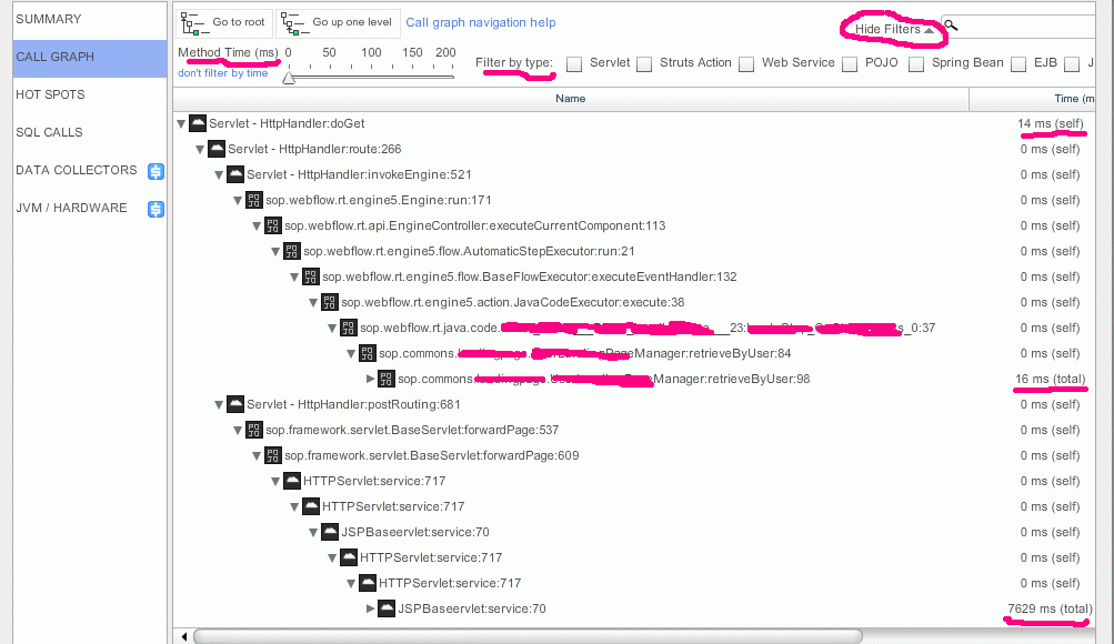
^Landing page will show list of recent transactions (web request) and highlight the response time in different color code depending on the settings (slow, very slow and stalling) which you can change at your own will. 


- Double-click the page name (URL) in red color and until you see the full call graph & timing of each spending.


    * First, it will drill down to all sampling of the same transaction (web request) 
   * Chose one of them and double-click to drill down to call graph
    ^you can filter the graph by method timing spending and class type (servlet, pojo, spring bean, ejb and etc)  
    
   *Click and click ... until you see something you are familiar 
    ^Take note of color code, don't confuse the total time spending (ORANGE) with method self time spending (BLUE)

As recent transactions are not good enough, we need to check out long transaction in past 30 minutes or 1 hours. Never mind, go and visit SnapShot page.

   * Click on SnapShot Tab
   ^ Too much info in the page, never mind, enable filter to view less and more concerned transactions.

    * Double-click the long transaction to pull out the call graph
   ^ There is JDBC call in this transaction

    * Right click on slow method to further expend the graph

   * Click on JDBC to check out list of executed SQL & time spending 

    * Scroll Up & Down and check what are the SQL and how much they spend in the total timing. 
    
   * Save the call graph for offline or offsite study by other developers  

    * Save to local disc and sent it to developers for further study. 
    ^ This file also includes list of executed SQL and timing of each.   

That is all, it is sweet & easy experience. In fact, i have put it up behind an Apach Server so that our offsite team can access and check out root cause of long transaction. 

Sunday, July 22, 2012

Java Heap, Stack Size, Perm Gen and Full GC tunning


A good start to understand JVM, Heap, Perm Gen and GC collector


GC Collector:


Serial Collector (-XX:+UseSerialGC)
• Throughput Collectors
> Parallel Scavanging Collector for Young Gen
 -XX:+UseParallelGC
> Parallel Compacting Collector for Old Gen
 -XX:+UseParallelOldGC (on by default with ParallelGC in JDK 6)
• Concurrent Collector
> Concurrent Mark-Sweep (CMS) Collector
 -XX:+UseConcMarkSweepGC
> Concurrent (Old Gen) and Parallel (Young Gen) Collectors
 -XX:+UseConcMarkSweepGC -XX:+UseParNewGC
• The new G1 Collector as of Java SE 6 Update 14 (-XX:+UseG1GC)

Sample JVM Parameters:


Performance Goals and Exhibits
A) High Throughput (e.g. batch jobs, long transactions)
B) Low Pause and High Throughput (e.g. portal app)
• JDK 6
A) -server -Xms2048m -Xmx2048m -Xmn1024m -XX:+AggressiveOpts
-XX:+UseParallelGC -XX:ParallelGCThreads=16
B) -server -Xms2048m -Xmx2048m -Xmn1024m -XX:+AggressiveOpts
-XX:+UseConcMarkSweepGC -XX:+UseParNewGC -XX:ParallelGCThreads=16
• JDK 5
A) -server -Xms2048m -Xmx2048m -Xmn1024m -XX:+AggressiveOpts
-XX:+UseParallelGC -XX:ParallelGCThreads=16 -XX:+UseParallelOldGC
-XX:+UseBiasedLocking
B) -server -Xms2048m -Xmx2048m -Xmn1024m -XX:+AggressiveOpts
-XX:+UseConcMarkSweepGC -XX:+UseParNewGC -XX:ParallelGCThreads=16
-XX:+UseBiasedLocking


Rule of Thumb on Best selection of

> Garbage Collector (Make sure to override GCThreads)
> Heap Size (-Xms == 1/64 Max Memory or Max Heap and
-Xmx == ¼ Max Memory or Max Heap)
> Runtime Compiler (-server vs -client)
• Desired Goals (This is a hint, not a guarantee)
> Maximum Pause Time (-XX:MaxGCPauseMillis=)
> Application Throughput (-XX:GCTimeRatio= where
Application time = 1 / (1 + n))

Do check out 1.5 paper as it comes with sample parameters for high thoughput and low latency application


If you are using 1.6, check out the difference and improvement from 1.6 paper, take note that 1.5 parameters still apply to 1.6.


A very practical and easy to understandable slide which walking you through the Sun HotSpot GC tuning tip and take-away parameters.


Wondering whether java thread stack space (Xss) and  perm gen (MaxPermSize) part of heap space. The answer is NO. That is why when u saw actually linux memory consumption is bigger than your "-Xmx" settings.

One working jvm parameters with JBoss server:

JAVA_OPTS="-server -Xms3072m -Xmx3072m -Xmn2048m -XX:MaxPermSize=256m -Dorg.jboss.resolver.warning=true -Dsun.rmi.dgc.client.gcInterval=3600000 -Dsun.rmi.dgc.server.gcInterval=3600000 -XX:ParallelGCThreads=8 -XX:+UseConcMarkSweepGC -XX:+UseParNewGC -XX:SurvivorRatio=8 -XX:TargetSurvivorRatio=90 -XX:MaxTenuringThreshold=31 -XX:+AggressiveOpts -XX:+PrintHeapAtGC -XX:+PrintGCTimeStamps -XX:+PrintGCDetails -XX:+PrintGCApplicationStoppedTime -Xloggc:/opt/jbos/server/default/log/jvmgc.log"


You have short-term memory on Linux Shell? Never mind, just check out this article and refresh your mind. 

Wednesday, July 4, 2012

Load Testing


Peak Hourly Visits and Average Visit Length

Peak Hourly Pages, Testcase Size and Duration

How Many Rows of Data Do I Need?


Recommend Readings

Oracle Archive Logging

[Original PostBasically, any change that happens in the database is first captured in a memory structure called the Log Buffer. This memory structure exists inside the Oracle Instance. The Log Buffer normally has a small footprint (somewhere in the neighborhood of 1MB). Information in the Log Buffer memory is flushed to the Redo Logs by the background process LGWR under these curcumstances:
a) every 3 seconds
b) on a commit
c) when the Log Buffer becomes 1/3 full
d) on a checkpoint

Anytime a) b) c) or d) occurs in the database, the information from the Log Buffer is written to the current Red Log by LGWR. Redo Logs are actual physical files residing on the OS. When a Redo Log becomes full, a Log File Switch occurs and a pointer is set to start writing Log Buffer information to the next Redo Log in line. You can run your database with only 2 Redo Logs, but Oracle (and common sense) recommends at least 3. 
So, after this Log File Switch, you have a Redo Log that is full and a pointer to the next Relo Log. The Redo Log that is full needs to be archived (saved somewhere else). So now, a background process called ARCH will get a nudge from LGWR saying "hey, got a redo log that needs to be archived" and ARCH will pick it up and convert it to an Archived Log file and save it in the location specified by your init.ora parameter setting called log_archive_dest_1 (or in yor flash_recovery_area, depending).
So now that the previous Redo Log has been archived, it can be overwritten by LGWR when necessary (e.g., Redo Logs are written to in a round-robin fashion and when Redo Log #3 fills up, the pointer goes back around to Redo Log #1. So if you're in archivelog mode and redo log #1 hasn't been completely archived by ARCH yet, and LGWR needs to write to Redo Log #1, then your database "hangs" until that Redo Log #1 is freed up to be written to again).

So, what is the advantage of having Archived Logs? Say for example you expereince severe corruption or a database crash that required you to restore some datafiles from 7 hours ago. If you have all the archived logs from that pint in time (7 hours ago) up until the oment of the crash, you can apply (or "roll forward") all the changes contained in those archived logs against the restored datafiles. Basically this replays all the changes in the database over the past 7 hours. After recovering the last archived log, Oracle will then look to roll forward even more by using the online redo logs. If those online redo logs contain changes necessary, Oracle will apply those changes also. Basically, you can recover from a serious error all the way up to just before the error occurred. Minimal data loss is the advantage here. you can't do this when you're not in archivelog mode, because all the changes over the past 7 hours are lost because the redo logs just keep overwriting themselves and all the changes are lost between the time of your last backup and the time of the crash.
As the mantra goes . . . if you don't care if your database loses data, then run in noarchivelog mode. If you care about your data and don't want to lose it, then run the database in archivelog mode.

Memory, Swap, Process, Thread, File, Data Storage and Tunning


Physical and virtual memory

Traditionally, one has physical memory, that is, memory that is actually present in the machine, and virtual memory, that is, address space. Usually the virtual memory is much larger than the physical memory, and some hardware or software mechanism makes sure that a program can transparently use this much larger virtual space while in fact only the physical memory is available.

Nowadays things are reversed: on a Pentium II one can have 64 GB physical memory, while addresses have 32 bits, so that the virtual memory has a size of 4 GB. We'll have to wait for a 64-bit architecture to get large amounts of virtual memory again. The present situation on a Pentium with more than 4 GB is that using the PAE (Physical Address Extension) it is possible to place the addressable 4 GB anywhere in the available memory, but it is impossible to have access to more than 4 GB at once.


Swap Space


Linux divides its physical RAM (random access memory) into chucks of memory called pages. Swapping is the process whereby a page of memory is copied to the preconfigured space on the hard disk, called swap space, to free up that page of memory. The combined sizes of the physical memory and the swap space is the amount of virtual memory available.


Linux has two forms of swap space: the swap partition and the swap file. The swap partition is an independent section of the hard disk used solely for swapping; no other files can reside there. The swap file is a special file in the filesystem that resides amongst your system and data files


How big should my swap space be?


Linux and other Unix-like operating systems use the term "swap" to describe both the act of moving memory pages between RAM and disk, and the region of a disk the pages are stored on. It is common to use a whole partition of a hard disk for swapping. However, with the 2.6 Linux kernel, swap files are just as fast as swap partitions. Now, many admins (both Windows and Linux/UNIX) follow an old rule of thumb that your swap partition should be twice the size of your main system RAM. Let us say I've 32GB RAM, should I set swap space to 64 GB? Is 64 GB of swap space really required? How big should your Linux / UNIX swap space be?


taskset  -p 
i.e.
taskset 1 -p 12345
to set process 12345 to use only processor/core 1
The bitmask can be a list (i.e. 1,3,4 to use cores 1 3 and 4 of a 4+ core system) or a bitmask in hex (0x0000000D the 1,3,4, 0x00000001 for just core 1)
taskset is usually in a package called shedutils.
Edit: almost forgot... If you want to set the affinity of a new command instead of change it for an existing process, use:
taskset   []...[]


Maximum number of threads per process in Linux

number of threads = total virtual memory / (stack size*1024*1024)

Java Process & Thread Limit on Linux

Maximum threads managed by java


Heap size                                                                                            

Java Heap size does not determine the amount of memory your process uses

If you monitor your java process with an OS tool like top or taskmanager, you may see the amount of memory you use exceed the amount you have specified for -Xmx. -Xmx limits the java heap size, java will allocate memory for other things, including a stack for each thread. It is not unusual for the total memory consumption of the VM to exceed the value of -Xmx.


Garbage collection


There are essentially two GC threads running. One is a very lightweight thread which does "little" collections primarily on the Eden (a.k.a. Young) generation of the heap. The other is the Full GC thread which traverses the entire heap when there is not enough memory left to allocate space for objects which get promoted from the Eden to the older generation(s).

If there is a memory leak or inadequate heap allocated, eventually the older generation will start to run out of room causing the Full GC thread to run (nearly) continuously.

The amount allocated for the Eden generation is the value specified with -Xmn. The amount allocated for the older generation is the value of -Xmx minus the -Xmn. Generally, you don't want the Eden to be too big or it will take too long for the GC to look through it for space that can be reclaimed.

´